TEXT

Over the past two decades, Rodney Stark and various associates have developed a rather unique approach to understanding religious behavior.[1]  Basing themselves at the intersection of exchange theory, micro-economics, and rational-choice approaches to individual agency, they have claimed that one can think of a society’s religious landscape as a marketplace.  In that marketplace, religious “firms” (churches) attempt to attract “customers” (members) for their religious “goods” – the beliefs, ideals, rituals, and social connections that are religions’ stock-in-trade.  Like Adam Smith (1776), Stark and associates argue that religious monopolies suppress trade and that religious competition enhances it.[2]  Leaving aside all its nuances, the approach explains Europe’s declining church attendance as the aftereffect of that region’s state-sponsored religions and America’s relative religiosity as the result of that country’s free religious market.  (Such a broad brush fails to do justice to Stark et al’s views, but the point here is to identify the approach, not to erect a straw man for later burning.)

Stark and his associates connect the overall shape of the religious marketplace with a series of individual choices – choices that they insist are quite rational.  They point out that religious behavior, like all other human behavior, is carried out by individuals.  Individuals clearly decide whether to attend church, which church (or churches) to attend, how often to pray, and so on.  People weigh such choices against alternatives.  Should one go to synagogue on Saturday or to the soccer game?  Should one donate to the fund for the new cathedral or send money to the soup kitchen.  Or, to take a situation in which there is much less religious freedom, should one stop work to pray along with one’s co-religionists, or risk being shot for failing to do so?  Empirically, each of these questions is a matter for individuals to decide.  On the face of the matter, it is rather plausible to these individuals pay some rational attention to the personal benefits and costs each choice brings.

The case gets more interesting.  Building on the previous work of Stark and Bainbridge (1987), Stark and Finke (2000) have developed this approach into a rather large number of supposedly testable propositions.  Covering everything from individual relationships with the supernatural to the shape of the religious landscape, these propositions systematize much previous sociological work.  Though some propositions are so unproblematic as to be almost definitional,[3] others are prima facie open to empirical verification.  For example, one can easily imagine a research project that tests Stark and Finke’s “Proposition 40: Mixed religious marriages are more likely to the degree that one or both spouses lack religious capital” (2000:124).

The propositional approach has two supreme virtues.  First, it is clear.  Based on a limited number of definitions and axioms, it makes predictions about both individual and group behavior.  These predictions’ testability puts science at the heart of the social-scientific study of religion – one of Stark’s oft-stated goals.  Second, it connects individual actions with overall social patterns, thus bridging the micro-macro divide that has long bedeviled sociology.  Stark and Finke write:

We begin at the micro level of analysis, with the individual, and build up the larger structures – many of which will emerge as we aggregate more micro processes. … We assemble a micro theory of religion that serves as the foundation for all the subsequent theorizing.  (2000:21-22)

In short, Stark and Finke produce what amounts to a unified field theory of religion’s human side.  Their approach grounds religious group dynamics in individual action.  And it claims to draw a direct connection between the actions of individuals and the dynamics of the group.

The present article tests the viability of this approach by taking it absolutely seriously.  It subjects Stark and Finke’s propositions to immanent analysis, by checking to see whether their account of individual religious choices actually generates the religious landscape that they predict.  Put more simply: Do the principles of individual religious action put forth by Stark et al. actually produce the aggregate-level behavior that they claim?  Or does something else result?  Stark and associates have always assumed a direct connection between individual choice and group outcomes.  As we shall see, the situation is more complex.

Schelling-Models

The technique that I shall use for this test is a Schelling-model – named after Thomas C. Schelling, who developed the method in the 1960s (1969; 1978).  A Schelling-model amounts to a thought-experiment, which connects individual action with group behavior by taking the interactions between individuals into account.  As we all know, people act not only based on what they want; they also act based on other people’s actions.  Often, such actions and actions upon actions generate aggregate results that bear little resemblance to any of the actors’ wishes.  Schelling-models allow one to visualize such patterns, cleanly.[4]

Let’s look at a simple example.  Take a computer-generated neighborhood, consisting of 144 possible house sites, inhabited by two types of people, the Reds and the Greens.  The neighborhood wraps left-to-right and top-to-bottom, so that each person is next to 8 lots on which neighbors can live.  Assume that the Reds are the majority – there are 60 of them – and the Greens are a minority of 25.  If we place these people randomly on our house sites, the neighborhood will look like the following.[5]  .

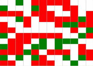
60 Reds, 25 Greens – Randomly Assigned

Furthermore, let us assume that both Reds and Greens favor housing integration.  Each “person” would like to live in an integrated neighborhood.  None, however, wants to live in isolation, surrounded by the other color.  Reds, being the majority, would like to have at least three Red neighbors.  Minority Greens would like at least two Green neighbors.  This means that each Red is happy living next to as many as five Greens and each Green is happy living next to as many as six Reds.  Everyone is happy being a local minority – just not too small of a minority.

Clearly, nearly all the Reds and Greens are satisfied with their starting living arrangements.  The neighborhood is nicely integrated, most Reds have at least three Red neighbors, and most Greens have at least two Green neighbors.  But not everyone is happy.  The leftmost Green in the second-to-the-bottom row is isolated, as are the two Greens in row 2.  The rightmost Red on row 2 has only one Red neighbor (remember that the neighborhood wraps left-to-right), and that neighbor, the leftmost Red, has only two Red companions.  Clearly, some people will want to improve their situations.

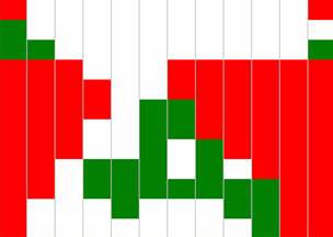
Now let’s let the dissatisfied people move, either until everyone is happy or until no one can improve her or his situation by shifting residences.  After seven rounds of moves, we end up with the following stable pattern:

After 7 Rounds, in Each of Which Everyone Gets a Chance to Move

The neighborhood is now segregated.  Everyone is now happy, at least insofar as no Red or Green is isolated among the other color.  But residential integration has vanished.  Though random placement at the start assures that each run of the simulation will be somewhat different, letting each Red or Green move to improve his or her lot always generates segregation.   Each Red or Green is willing to be a minority among its neighbors, even a small minority.  If the members of both groups specify that they must not be isolated, however, the two groups divide. 

Scholars have spent the last generation confirming this result – for almost any size groups, any residence requirements, and any dimensions of social division.  Though none of our Reds or Greens is personally “colorist” – i.e., bigoted against the other group – any degree of residential preference results in group separation.  Schelling does not deny the presence of racism in American life (for segregation by race stimulated his model).  But he shows the unintended consequences of individual choices for the patterns of group behavior.  Jonathan Rauch (2002) quotes Schelling’s 1969 Rand Corporation report:

The interplay of individual choices, where unorganized segregation is concerned, is a complex system with collective results that bear no close relation to the individual’s intent. 

Rauch goes on to note that

Even in this extremely crude little world, knowing individuals’ intent does not allow you to foresee the social outcome, and knowing the social outcome does not give you an accurate picture of individuals’ intent.  Furthermore, the godlike outside observer – Schelling, or me, or you – is no more able to foresee what will happen than are the agents themselves.  The only way to discover what pattern, if any, will emerge from a given set of rules and a particular starting point is to move the pennies around and watch the result.[6]

Simulating the Religious Landscape

To my knowledge, no one has yet used Schelling-models to see the aggregate results of individual religious choices.  I have recently written a computer program to do so, which is available for download at my university’s website. [7]  It begins with a landscape of 10,000 individuals, each with a religious preference (or a preference for no religion at all).  One sets various rules by which individuals make decisions, patterned on Stark et al’s claims about the choices that religious individuals make.  One then runs the simulation, letting each of the 10,000 individuals choose to keep her or his current religion, convert to another religion, or abandon religion altogether.  

Patterns emerge in the religious landscape, as we shall soon see.  Those patterns allow us to test Stark and Finke’s (2000) propositions about such landscapes.  If their individual-level decision rules produce their predicted aggregate-level results, then we can conclude that their model works – in the laboratory, if not in real life.  If, on the other hand, the aggregate picture fails to match their predictions, we know that their model does not work at all.

I deliberately use the word “model” rather than the word “theory” here, for reasons that I explain below.  I further emphasize that this is not an empirical test of Stark and Finke’s approach.  Like Schelling’s work, it is a thought-experiment.  If people acted as Stark and Finke claim they act, would we actually get the results that they predict?  Or would we get something else?  Let us see.

Setting the Starting Religious Landscape

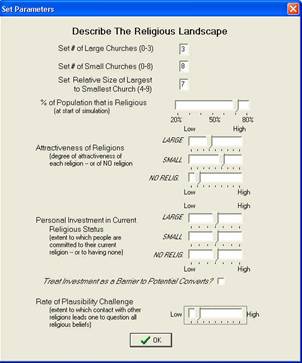
We begin the simulation by setting the starting characteristics of the religious landscape, as follows:

§         The number of large religions, the number of small religions, and the relative size difference between these large and small groups.  (Stark et al. claim that large, lazy churches act differently than small, hungry ones, so we need to see what happens with each type under various scenaria.)

§         The percent of the total population that belongs to religious groups.

§         The attractiveness of each size religion to outsiders – which can also be read as the degree to which individual churches actively woo converts.  (This can be set differently for large churches than for small ones.)  Also the general attractiveness of having no religion.  We can think of this as the degree to which general social processes make church membership unattractive – perhaps because the prevailing culture teaches one that it is more fun to spend Sunday at the beach. 

§         The degree of personal investment that individuals have in their current religion – this, too, can be set differently for large and small churches – and also in having no religion.

§         Whether this degree of investment will merely encourage individuals to stick with their current religion, or whether it will also form a possible barrier to newcomers.  In the first case, those belonging to high investment groups will not likely convert, but the degree of investment required of members will not influence those who wish to join.  If the box is checked, outsiders will be less likely to join a group that requires high commitment – even though they are more likely to stay in such a group, once they have joined.
            This factor is equivalent to a group’s tension with its surrounding environment.  With the box checked, high-investment groups will be less likely to gain members from or lose members to low-investment groups and/or the secular world.[8] 

§         The degree to which an individual’s exposure to a large number of competing religions leads her or him to question the validity of them all.  This tests Peter Berger’s (1969) thesis that religious pluralism increases agnosticism – and thus decreases religious membership.  (Other kinds of “secularization” can be imitated by making irreligion more attractive.)

Having set these parameters, the simulation then produces a visual representation of the religious landscape.  Individuals are randomly assigned to various groups, based on the number of churches, the relative size of large and small churches, and the percent of the population belonging to any church at all.  (The other factors generate the rules for potential conversion, and so do not affect the starting point.)  For example, specifying 3 large churches, eight small churches, a 1/7 size ratio with 70% of the population religious gives us this starting point:

A Diverse Religious Landscape

The column on the right reminds us of the starting conditions.  The key on the left tells us how many members belong to each of the variously colored churches.  The former stays constant throughout the exercise; the latter changes as people convert from one religion to another.

What happens as we let people change religions, abandon religion, or stay where they are?  Here are the results after 2, 5, 10, and 100 cycles:

As you can see, religious competition changes the religious landscape quite radically. 

The first thing that we notice in this case is that church members clump together almost immediately.  Unlike the “Choosing Neighbors” simulation, this does not involve them moving from one house to another, to be with like-minded neighbors.  Instead, one’s neighbors can bring about one’s religious conversion – under certain circumstances.  For example, if one belongs to the Red faith, but one is surrounded by Blues – and if those Blues’ collective attractiveness outweighs one’s own investment in Redness – then one converts. 

Each person has eight religious neighbors, each with her or his own religious preference.  If three or four of those neighbors belong to a single church, that church’s attractiveness multiplies – usually enough to overcome one’s own loyalties.  Joining the neighbors’ church thus produces a small cell.  The rules of the game make it almost impossible to convert someone surrounded by co-religionists, so these cells grow and shrink at the edges.  Sooner or later – usually after 50 or 100 rounds, the religious landscape becomes stable, with clumps of like-minded persons having replaced the random pattern with which we began.

The production of such groups results from the simulation’s conversion algorithm.  My program follows Stark’s long-held view that conversion takes place through the medium of social ties (Lofland and Stark.1965; see also Stark and Finke. 2000:chapter 5).  In this view, people convert because of their social contacts. [9]  The program treats each individual as having eight such contacts – instanced as the eight squares with which individual is surrounded.  In real life, some of those contacts might be virtual: being connected with someone by the Internet is no different mathematically than being connected with someone at work or being connected with someone living next door. 

In effect, clumping tells us that – all other things being equal – converting to the religion of one’s neighbors reduces one’s religious ties to members of other groups.  Indeed, it does so quite rapidly.  Nearly all of the simulations that I present here show people quickly limiting their religious contacts with outsiders.  This does not mean that people cut all of their social ties, because the simulation models religious contacts – or at least those contacts that could lead one toward conversion.  Just as the “Choosing Neighbors” simulation did not take into account people’s preferences for housing style, plumbing quality, and so on, so our religious simulation does not take into account one’s non-religious relationships.  Each person’s eight neighbors stand for eight potential religious contacts.  It is those contacts that quickly become limited.

But not for everyone. If we change just one parameter for our starting point – by raising each individual’s investment in her or his current church from 5 to 6 (for both large and small religions), we get the following results:

As you can see, the clumping is minor and stops rather quickly; in fact, there is typically no movement after 7-10 cycles.[10]  Such tipping-points are rather common in Schelling-models, as small differences in individual decision-rules lead to vastly different social equilibria.

So, clumping results whenever people’s openness to conversion outweighs their attachment to their current faith.  People who are highly attached can have religious relationships with quite disparate others, because they will not be tempted to convert.  Where this is not the case, however, a society in which individuals have religious choice, and in which their religious neighbors influence that choice, results in (relative) religious encapsulation.  Such a “sectarian” result occurs in large churches as well as in small ones. 

Clumping thus does not model tension with society; we set that separately by treating religious attachment as a barrier to outsiders as well as to one’s own conversion.  Limiting one’s religious contacts seems to be a natural result of being open to religious change.  Groups that encapsulate themselves quickly expand, while those that fail to do so decline.

Now look back at our original scenario.  There, the only consistent loser in these four charts was the “group” that had no religion.  Most runs with the above settings soon reduce these “seculars” to a few or none – 35, in the case here illustrated.  This, too, is a natural outcome of the settings with which the simulation began.

Remember that we set the attractiveness of having no religion at one, the attractiveness of large religions at three and the attractiveness of small religions at five.  Large churches are three times as attractive as having no religion, and small churches are five times as attractive.  (The large-small discrepancy matches Stark et al’s claim that small churches do a better job of wooing members than do large churches.)  We have given all three groups an equal investment in their current choice.

In these circumstances, it makes sense that people with “no religion” would join a church, because we have specified that having “no religion” is much less attractive than having one.  What does not make immediate sense is the continued dominance of larger churches in this religious landscape.  Our settings, remember, make small churches more attractive than large ones.  Why doesn’t this produce the same results on the aggregate level?

In our example, the Blue group – one of the original large churches – has grown to nearly twice its original size.  Of the other large churches, the Green group has neither gained nor lost members and the Red group has shrunk by about half.  Most of the small churches – Yellow, Aqua, Lime, Fuschia, Purple, and Navy – have grown, though they are still smaller than the originally large groups.  The Maroon church has nearly disappeared and the Teal and Navy churches have barely kept their original numbers.

Running the simulation with these parameters intact, but with different random starting assignments, generates results with the same overall pattern.  People with “no religion” disappear, one of the large churches grows, at least one of the other two large churches stays large, most of the small churches grow – but not to the level of the original large churches – and at least one of the small churches disappears.

Clearly, there is no direct and unequivocal connection between a church’s marketing efforts (its attractiveness) and its growth.  Therefore, we cannot argue directly from individual choices to social outcomes.  Large religious organizations apparently do not need to work as hard to maintain or increase their market share as do small groups, and hard work is no guarantee of success, even if all other things are equal.  For that is the point of this simulation: to keep everything equal except the specific variables that we wish to test.

Enough of an introduction!  There are 364,568,526 different ways to set this simulation’s parameters, many of which have direct relevance to Stark et al’s model of religious markets.  For reasons of space, I shall explore only one topic here (though it will take several simulations for me to do so).  Specifically, I shall test two of Stark and Finke’s propositions about the factors influencing the shape of religious landscapes.  These are:

Proposition 72: The capacity of a single religious firm to monopolize a religious economy depends upon the degree to which the state uses coercive force to regulate the religious economy.

Proposition 75: To the degree that religious economies are unregulated and competitive, overall levels of religious commitment will be high.  (Conversely, lacking competition, the dominant firm[s] will be too inefficient to sustain vigorous marketing efforts, and the result will be a low overall level of religious commitment ….)

Both of these propositions are open to simulative testing.

Marketing and Market Share

To test Proposition 72, I shall start with a simple case:  there is just one religion, its members make up some variable percentage of the population, and everyone else is non-religious.  If we change none of the other basic settings – i.e., if belonging to that church is three times as attractive as belonging to no religion at all, and if both religious and non-religious people are equally attached to their views – then repeated testing shows that it takes at most six cycles for everyone to join the religion in question.  This is true, no matter how much that religion has to grow in order to encompass the whole landscape.  As you can see from the left-most cell in the chart below, even a church that starts at only 20% of the population will convert everyone in short order!

Why?  Actually, the simulation doesn’t tell us.  It is entirely a matter of the differential attractiveness of our one religion and of having no religion at all.  This might involve state coercion, but it might also involve good religious marketing, or even the lack of attractive non-religious activities.  For example, perhaps non-religion is attractive because people like to go to the beach on Sunday.  What if the beaches were all in Greenland or on Baffin Island?  Even the hardest pews might then look comfortable.  It is thus not necessarily state coercion that produces religious monopoly; the lack of competition plus a three-times differential attractiveness can do so as well.

To generate the two right-most cells in this chart, I have lowered the attractiveness of our one religion by one notch, thus changing the attractiveness ratio between our one religion and having no religion at all.  Running the simulation with 20% of the population belonging to a church produces no change!  After 50 cycles, 20% of the population is still religious and 80% is still irreligious, though there have been some conversions.  Running repeated simulations at 30%, 40%, etc. of the population belonging to our one church gradually increases that church’s reach.  A 50% starting point results in 60% church membership – but no more, even after 50 cycles.  An 60% starting point results in nearly 90% church membership.  A church apparently has to be more than twice as attractive as having no religion, and it must have a significant social presence, if it is to dominate the religious landscape. 

There is, of course, one more ratio to consider: between the attractiveness of a given religion and each person’s investment in her or his current situation.  Playing with this slider generates several interesting patterns, two of which I reproduce below. 

Fifty cycles of the left-hand simulation results in a stable religious landscape in which 35% belong to the Blue Church.   Five cycles of the right-hand simulation results in complete conversion.   This is a tipping point: a spot were a small shift in a single parameter makes a huge difference in outcomes.  Such points are common in Schelling-models, and often highlight important social patterns.  As we shall see, our simulation produces many such tipping points.   None of them is predicted by the Stark-Finke propositions.

If religion and irreligion are equally attractive, by the way, we get another tipping point.  Let’s assign both our one church and no-church an attraction of 3, and vary the starting percentage religious. 

Both simulations reach stability within the first 50 cycles, shifting only slightly thereafter.  Clearly, the percentage of the population that is religious when we begin the simulation has a great deal of effect of the outcome.

What does all this say about Proposition 72?  Clearly, there seems to be more than one route to a single church dominating the religious landscape.  Religious dominance requires state aid only if the lone church is almost completely incapable of selling itself to outsiders, and if it also does not have much of a religious presence.  The individual-level religious choices on which Stark and Finke’s system supposedly rests do not require us to assume such things.

Among other things, this tells us that Stark and Finke’s Proposition 72 is much too simple.  The “capacity of a single religious firm to monopolize a religious economy” – or even to dominate it – depends on its relative attractiveness vis-à-vis the non-religious alternative, the ratio of that attractiveness to the investment that individuals have in their religiosity or their irreligiosity, and – above all – on the percentage of the population that is religious at the start of the exercise.  It is this last factor that proves to be the most sensitive.

Yes, state coercion may play a role.  But it is not the only factor.

Competition

The immediately preceding simulations have involved a single religion, and we explored the circumstances under which that religion comes to dominate the religious landscape.  Now let’s introduce some religious competition. 

Seeding our starting landscape with one large church and five small ones, each equally attractive (and each three times as attractive as the non-religious alternative), always results in the one large church taking over the entire religious landscape.  This happens no matter how we set the starting religious percentage: even if we begin with just 20% of the population religious, it only takes between 75 and 125 cycles for the entire field to convert to Blue; at 80%, ten cycles usually does the trick.  Raising the attractiveness of no religion one notch (to a 3/2 ratio with large religions) produces a tipping point: above 35%, everyone joins the Blue church; below 35%, at least 85% lose religion altogether.  Making small churches, large churches, and no religion equally attractive shifts the tipping point to 75%.[11]

As you can see, the Blues dominate.  When both large and small churches are equally attractive, the large ones have a competitive advantage.  (But not all scenaria result in increased religious penetration.)  Now let’s try three large religions – thus equalizing the competitive playing field.  All are equally attractive, but now none has the advantage of size.

As you can see, they may start out equally, but they don’t end that way.  The results differ for various ratios of attraction vis-à-vis no religion, but above each tipping point we get a single dominant religion. Clearly, competition alone does not reduce a single church’s dominance of the religious field.

Now we turn back to our previous example: one large religion and several small religions at various starting religious percentages.  We have already learned that the attraction ratio between church and no church matters.  How much more attractive do we have to make small churches than large churches, to avoid one large church dominating the religious landscape?

Here are three among many possibilities.  Each simulation began with a 60% religious/40% non-religious population, with one large church and five small ones, and with large churches three times as attractive as no religion.  All I have varied are the attractiveness ratios of the large and small churches: 3 to 4, 3 to 6, 3 to 8.

Clearly, small churches have to outmarket their larger competitors in order to avoid being put out of business.   In general, they have to be twice as aggressive in their effort to gain converts.  Stark and Finke build this into their model (see the second half of Proposition 75), but they claim it as a result of individual choices.  Our simulations show that it must be an assumption of those choices, not a result.  Stark and Finke have mistaken results for assumptions, at least on this score.

Note that these results only hold if we make having no religion relatively unattractive.  As soon as we raise the attractiveness of the beach, the soccer game, or mass entertainment, we find another tipping point.  With large religions no more attractive than no religion, small religions must be at least twice as attractive as either to avoid religious decline.[12]

Let me reiterate that these are theoretical results, not empirical ones.  I have taken the claims that Stark et al make for individual religious action and set those claims in motion on a religious field.  The fact that the results do not match Stark and Finke’s predictions does not tell us anything about how the real-life religious economy operates.  Instead, they tell us that Stark and Finke’s assumptions about individual religious action produce a religious economy that does not match their predictions for it.  The connection that they draw between individual religious action and the shape of the religious market is incorrect.

Does Competition Produce Increased Religion?

Our next task is to examine the claim of Stark and Finke’s Proposition 75: that competitive economies will generate high “overall levels religious commitment”.  Indeed, Stark and Finke claim that competition generates higher levels of such commitment than does an uncompetitive situation. 

There are two ways to read this phrase.  Commitment might mean individual commitment – perhaps a greater dedication to an organization to which one already belongs.  Or it might mean greater religious participation – a higher level of total church attendance, religious membership, and so on.  Unfortunately, our simulation does not allow us to measure changes at the individual level.  It does, however, show us what percentage of the total population belongs to religious groups at each point in time.  I think it reasonable to use this collective measurement, given Stark et al’s previous claim of a relationship between religious competition in the U.S. and high levels of religious participation there, compared to Europe.  Our question then becomes, does a competitive religious environment generate more religious participation in toto?  Or are other factors involved?

Let me begin by drawing attention to the fact that increased religious participation can occur even when there is just one religion, as several of the above charts show.  A non-competitive marketplace can result in overall religious growth – or in the disappearance of irreligion, which amounts to the same thing.  Much depends on the ratio between the attractiveness of variously sized religions and the attractiveness of being irreligious.  Much also depends on the level of overall religiosity with which the market begins.

Moving forward, let us separate starting situations in which there are a large number of equally-sized religions from those in which there are one or two large religions and a group of small ones. 

We’ll first choose 8 equal-sized religions, to see under which circumstances we get overall religious growth and overall religious decline.  Our next chart compares six related scenaria.  For each, the “Ratio =” shows the ratio between the attractiveness (or marketing skill) of each of the religions and the attractiveness of having no religion at all.  The first percentage in each label indicates the percent-religious with which the simulation started.  The second percentage is the percent-religious after the simulation achieves stability.  I have chosen typical cases, after running a rather large number of each simulation to identify trends. 

Like many of our previous examples, the attractiveness ratio makes a great deal of difference to the model’s outcome.  The charts I show here identify tipping points at various ratio levels. 

Even at the lowest possible level of religious participation – i.e., at the highest possible level of irreligion – a 5/1 attractiveness ratio increases overall religious participation to 50%.  This is as far as it goes; running the simulation longer does not produce any more religious penetration.  (This has to do with the clumping phenomenon we found at the very beginning of this exercise.)

At 5/2, where having no religion is more attractive than before, but still considerably less attractive than belonging to any of the religious groups, 20% religious penetration produces stability.  If we start with 20% of the population being religious, we end with 20% religious.  One of our churches, however, puts the others pretty much out of business.  Almost all of those who remain religious become Green.  If we start with 30% religious penetration, however, we quickly rise to 65% with much more equal numbers.  This particular simulation supports Stark and Finke’s model.

The situation is similar, but more extreme, where the ratio is 5/3.  Though having a religion is still significantly more attractive than not having one, the overall percentage of the population that is religious falls when we start with only 60% religious penetration.  A starting-point at 70% quickly grows to 95%, however.  With the latter beginning level, irreligion seems doomed.

Lowering the ratio to 5/4 shifts the tipping point up the scale.  A starting 80% penetration rate falls to 30%.  It does not, however, fall beyond that, again because of clumping.  Forcing conversion to occur only between neighbors protects churches from random loss of members.  (One could develop a different conversion algorithm, of course, but doing so would violate the principles of Stark’s approach.)

The net result of this experiment is to show the overwhelming importance of religious attractiveness – or, looked at another way, of marketing skill.  Increasing a society’s overall level of religious participation requires more than just religious competition; it demands that the marketing efforts that such competition supposedly generates must be several times stronger than the marketing efforts of the secular “opposition”.  It is not enough for churches to outsell their competitors in the secular world; they must outsell them many times over. 

Note one more thing.  In three of the above simulations, at least one of the competing churches went out of business.  Its members converted to other faiths, while it failed to convert others in return.  This result had nothing to do with market efforts, because each of the 8 groups was given identical market skills.  Instead, market failure resulted from random assignment of individuals to the various religious (and non-religious) groups. 

Luck plays a part in every quest.  One cannot draw a straight line from actors’ resources and intentions to social outcomes. 

So much for pitting equal-sized churches against one another.  What happens to religious penetration if we seed our landscape with both large and small churches?  What if, additionally, we follow Stark et al’s suggestion that such large churches are less motivated to market themselves to outsiders than are smaller, “hungrier” groups – i.e., that their attraction level is lower?  Does this kind of competition generate increased religious participation overall, as Stark and his associates have long suggested?

The very first chart that I introduced above (on page 6) traced the results of seeding three large religions and eight small ones into a landscape that is 70% religious.  Assuming attractiveness scores of 1, 3, and 5 for no religion, large churches, and small churches, respectively, 100 cycles results in a 95% religious penetration rate.  The tipping point for this scenario is a starting religious penetration rate of 30%.  Higher than that, religion expands.  Lower than that, it declines.  If we change the attractiveness scores to 2, 3, and 5, the tipping point moves to 50% religious penetration.  A scenario begun at that level raises the religious participation rate to 70-75%; anything higher produces a saturated religious field.  Changing the scores to 3, 3, and 5 moves the tipping point to 80%.  Any starting point with less religious penetration than that results in religious decline.

We can, of course, raise the attractiveness score if the small churches.  Setting the scores at 3, 3, and 6 for no religion, large churches, and small churches moves the tipping point  down to 60%; 3, 3, and 7 moves it to 50%;  and 3, 3, and 8 moves it to 20%.  The more effort that small churches put into their proselytizing, relative to the efforts of large churches or the attractions of the beach, soccer, and Hollywood, the greater the total percentage of the population that ends up as church-goers. 

To a degree, then, Stark and Finke’s Proposition 75 is right.  If churches are sufficiently more attractive to potential converts than is the non-religious alternative, and if a sufficiently large percentage of the starting population is religious, then religious competition will increase the overall degree of religious participation.  There is, however, a tipping point for each attraction ratio.  If the starting percentage is below that tipping point, competition produces religious stagnation or even decline.  It is only above the tipping point that total religious participation grows.

A Note on “Models” and “Theories”

Some years ago, I published an article evaluating the rational-choice approach to religions as a theory of how religion works (Spickard 1998).  I built that essay around Lawrence Iannaccone’s clear and concise statement of the assumptions on which “a meaningful rational choice model of religion” can be be built.  As Iannaccone framed the matter,

Gary Becker has aptly characterized the "heart" of the rational choice approach as "the combined assumptions of maximizing behavior, market equilibrium, and stable preferences, used relentlessly and unflinchingly."  ...  Frankly, I cannot imagine a meaningful rational choice model of religion that does not ultimately rest upon these three assumptions:

§         Assumption #1: Individuals act rationally, weighing the costs and benefits of potential actions, and choosing those actions that maximize their net benefits.

§         Assumption #2: The ultimate preferences (or "needs") that individuals use to assess costs and benefits tend not to vary much from person to person or time to time

§         Assumption #3: Social outcomes constitute the equilibria that emerge from the aggregation and interaction of individual actions.  (Iannaccone 1997:26)

My critique of this approach showed that the first assumption is a possible retrospective reconstruction of individual action, but (demonstrably) it does not capture the actual thought processes that individuals follow in making decisions.  It showed that the second assumption is empirically false.  And it argued that the third assumption is questionable if read one way and is so vague as to be nearly meaningless if read another.  First, does everything result in true equilibrium?[13]  Second, what else might “social outcomes” be, other than the “aggregation and interaction of individual actions”?

Given this situation, I argued that the rational-choice model of religious action is not a “theory”, per se, but a “model”.  That is, it is an intellectual device that produces macro-level outcomes based on micro-level inputs.  Such devices do not necessarily mirror real social processes; instead, they mirror their aggregate results.  They are much like a chess-playing computer.  IBM’s “Deep Blue” beat Grandmaster Gary Kasparov at chess, but one cannot conclude from this that both Deep Blue and Kasparov think their chess in the same way.  Though it won its match, Deep Blue did not do so by mirroring human reasoning processes.  It used different techniques, much faster than any human could.  It took another route to winning. 

Theories tell us how things work; models reproduce the results of their working.  Thus, I concluded, the rational-choice approach to religious markets is not a “theory” of religious action, because it is demonstrably wrong in its account of how people actually act.  It is at most a ”model” that might mimic aggregate religious behavior. 

In the present article, I have called my own bluff.  I produced an actual model of the Stark-Finke-Bainbridge-Iannaccone approach to religion, one that tells 6-pixel-by-6-pixel blocks of computer screen to act according to the principles that these scholars claim for human agents.  I turned on that model, to see whether it actually produces the religious landscapes that Stark et al claim.

Leaving aside all of the nuances of the foregoing discussion, the overall answer is “no.”  The religious landscapes that Stark and Finke describe in various of their propositions do not result from the kind of individual, rational religious action that they claim occurs.  Whether or not empirical individuals follow rational-choice principles – as I previously argued they do not – a “society” of rationally-choosing computer agents does not produce the religious landscape that Stark and Finke claim it will.  Its results are much more complex and, I think, much more interesting.

I have not, of course, explored all 364 million simulations of which my program is capable.  In this article, I have not even described all of those that I have viewed.  Chief among these is a routine to test Stark and Finke’s predictions about the results of various levels of tension between religious groups and the societies in which they live.  I encourage other scholars to download this software, explore it, and publish their results.  Perhaps they will find more simulations that match Stark and Finke’s predictions than have I.

I also encourage scholars to find ways to apply Schelling-models to other aspects of social life. Though thought-experiments rather than empirical explorations, such models are powerful tools for testing both models and theories in the social sciences.